Section - 8 Evaluate Model Performance
Now we get to see the results of our hard work! There are some additional data preparation steps we need to take before we can visualize the results in aggregate; if you are just looking for the charts showing the results they are shown later on in the “Visualize Results” section below.
8.1 Summarizing models
Because we know what really happened for the target variable in the test data we used in the previous step, we can get a good idea of how good the model performed on a dataset it has never seen before. We do this to avoid overfitting, which is the idea that the model may work really well on the training data we provided, but not on the new data that we want to predictions on. If the performance on the test set is good, that is a good sign. If the data is split into several subsets and each subset has consistent results for the training and test datasets, that is an even better sign the model may perform as expected.
The first row of the data is for the BTC cryptocurrency for the split number 1. For this row of data (and all others), we made predictions for the test_data using a linear regression model and saved the results in the lm_test_predictions column. The models were trained on the train_data and had not yet seen the results from the test_data, so how accurate was the model in its predictions on this data?
8.1.1 MAE
Each individual prediction can be compared to the observation of what actually happened, and for each prediction we can calculate the error between the two. We can then take all of the values for the error of the prediction relative to the actual observations, and summarize the performance as a Mean Absolute Error (MAE) of those values, which gives us a single value to use as an indicator of the accuracy of the model. The higher the MAE score, the higher the error, meaning the model performs worse when the value is larger.
8.1.2 RMSE
A common metric to evaluate the performance of a model is the Root Mean Square Error, which is similar to the MAE but squares and then takes the square root of the values. An interesting implication of this, is that the RMSE will always be larger or equal to the MAE, where a large degree of error on a single observation would get penalized more by the RMSE. The higher the RMSE value, the worse the performance of the model, and can range from 0 to infinity, meaning there is no defined limit on the amount of error you could have (unlike the next metric).
8.1.3 R Squared
The \(R^2\), also known as the coefficient of determination, is a measure that describes the strength in the correlation between the predictions made and the actual results. A value of 1.0 would mean that the predictions made were exactly identical to the actual results. A perfect score is usually concerning because even a great model shouldn’t be exactly 100% accurate and usually indicates a mistake was made that gave away the results to the model and would not perform nearly as good when put into practice in the real world, but in the case of the \(R^2\) the higher the score (from 0 to 1) the better.
8.1.4 Get Metrics
We can return the RMSE and \(R^2\) metrics for the BTC cryptocurrency and the split number 1 by using the postResample() function from the caret package:
postResample(pred = cryptodata_nested$lm_test_predictions[[1]],
             obs = cryptodata_nested$test_data[[1]]$target_price_24h)
## RMSE Rsquared MAE
## 260.560193954 0.002833784 236.892256914We can extract the first element to return the RMSE metric, and the second element for the R Squared (R^2) metric. We are using [[1]] to extract the first element of the lm_test_predictions and test_data and compare the predictions to the actual value of the target_price24h column.
This model used the earliest subset of the data available for the cryptocurrency. How does the same model used to predict this older subset of the data perform when applied to the most recent subset of the data from the holdout?
We can get the same summary of results comparing the lm_holdout_predictions to what actually happened to the target_price_24h column of the actual holdout_data:
postResample(pred = cryptodata_nested$lm_holdout_predictions[[1]],
             obs = cryptodata_nested$holdout_data[[1]]$target_price_24h)
## RMSE Rsquared MAE
## NA 0.02235188 NAThe result above may show a value of NA for the RMSE metric. We will explain and resolve the issue later on.
8.1.5 Comparing Metrics
Why not just pick one metric and stick to it? We certainly could, but these two metrics complement each other. For example, if we had a model that always predicts a 0% price change for the time period, the model may have a low error but it wouldn’t actually be very informative in the direction or magnitude of those movements and the predictions and actuals would not be very correlated with each other which would lead to a low \(R^2\) value. We are using both because it helps paint a more complete picture in this sense, and depending on the task you may want to use a different set of metrics to evaluate the performance. It is also worth mentioning that if your target variable you are predicting is either 0 or 1, this would be a classification problem where different metrics become more appropriate to use.
These are indicators that should be taken with a grain of salt individually, but comparing the results across many different models for the same cryptocurrency can help us determine which models work best for the problem, and then comparing those results across many cryptocurrencies can help us understand which cryptocurrencies we can predict with the most accuracy.
Before we can draw these comparisons however, we will need to “standardize” the values to create a fair comparison across all dataasets.
8.2 Data Prep - Adjust Prices
Because cryptocurrencies can vary dramatically in their prices with some trading in the tens of thousands of dollars and others trading for less than a cent, we need to make sure to standardize the RMSE columns to provide a fair comparison for the metric.
Therefore, before using the postResample() function, let’s convert both the predictions and the target to be the % change in price over the 24 hour period, rather than the change in price ($).
8.2.1 Add Last Price
In order to convert the first prediction made to be a percentage, we need to know the previous price, which would be the last observation from the train data. Therefore, let’s make a function to add the last_price_train column and append it to the predictions made so we can calculate the % change of the first element relative to the last observation in the train data, before later removing the value not associated with the predictions:
last_train_price <- function(train_data, predictions){
  c(tail(train_data$price_usd,1), predictions)
}
We will first perform all steps on the linear regression models to make the code a little more digestible, and we will then perform the same steps for the rest of the models.
8.2.1.1 Test
Overwrite the old predictions for the first 4 splits of the test data using the new function created above:
cryptodata_nested <- mutate(cryptodata_nested,
                            lm_test_predictions = ifelse(split < 5,
                                                         map2(train_data, lm_test_predictions, last_train_price),
                                                         NA))
The mutate() function is used to create the new column lm_test_predictions assigning the value only for the first 4 splits where the test data would actually exist (the 5th being the holdout set) using the ifelse() function.
8.2.1.2 Holdout
Do the same but for the holdout now. For the holdout we need to take the last price point of the 5th split:
cryptodata_nested_holdout <- mutate(filter(cryptodata_nested, split == 5),
                                    lm_holdout_predictions = map2(train_data, lm_holdout_predictions, last_train_price))
Now join the holdout data to all rows based on the cryptocurrency symbol alone:
cryptodata_nested <- left_join(cryptodata_nested,
                               select(cryptodata_nested_holdout, symbol, lm_holdout_predictions),
                               by='symbol')
# Remove unwanted columns
cryptodata_nested <- select(cryptodata_nested, -lm_holdout_predictions.x, -split.y)
# Rename the columns kept
cryptodata_nested <- rename(cryptodata_nested,
                            lm_holdout_predictions = 'lm_holdout_predictions.y',
                            split = 'split.x')
# Reset the correct grouping structure
cryptodata_nested <- group_by(cryptodata_nested, symbol, split)
8.2.2 Convert to Percentage Change
Now we have everything we need to accurately calculate the percentage change between observations including the first one. Let’s make a new function to calculate the percentage change:
standardize_perc_change <- function(predictions){
  results <- (diff(c(lag(predictions, 1), predictions)) / lag(predictions, 1))*100
  # Exclude the first element, next element will be % change of first prediction
  tail(head(results, length(predictions)), length(predictions)-1)
}
Overwrite the old predictions with the new predictions adjusted as a percentage now:
8.2.3 Actuals
Now do the same thing to the actual prices. Let’s make a new column called actuals containing the real price values (rather than the predicted ones):
actuals_create <- function(train_data, test_data){
  c(tail(train_data$price_usd,1), as.numeric(unlist(select(test_data, price_usd))))
}
Use the new function to create the new column actuals:
cryptodata_nested <- mutate(cryptodata_nested,
                            actuals_test = ifelse(split < 5,
                                             map2(train_data, test_data, actuals_create),
                                             NA))
8.2.3.1 Holdout
Again, for the holdout we need the price from the training data of the 5th split to perform the first calculation:
cryptodata_nested_holdout <- mutate(filter(cryptodata_nested, split == 5),
                                    actuals_holdout = map2(train_data, holdout_data, actuals_create))
Join the holdout data to all rows based on the cryptocurrency symbol alone:
cryptodata_nested <- left_join(cryptodata_nested,
                               select(cryptodata_nested_holdout, symbol, actuals_holdout),
                               by='symbol')
# Remove unwanted columns
cryptodata_nested <- select(cryptodata_nested, -split.y)
# Rename the columns kept
cryptodata_nested <- rename(cryptodata_nested, split = 'split.x')
# Reset the correct grouping structure
cryptodata_nested <- group_by(cryptodata_nested, symbol, split)
8.2.4 Actuals as % Change
Now we can convert the new actuals to express the price_usd as a % change relative to the previous value using adapting the function from earlier:
8.3 Review Summary Statistics
Now that we standardized the price to show the percentage change relative to the previous period instead of the price in dollars, we can actually compare the summary statistics across all cryptocurrencies and have it be a fair comparison.
Let’s get the same statistic as we did at the beginning of this section, but this time on the standardized values. This time to calculate the RMSE error metric let’s use the rmse() function from the hydroGOF package because it allows us to set the na.rm = T parameter, and otherwise one NA value would return NA for the overall RMSE:
hydroGOF::rmse(cryptodata_nested$lm_test_predictions[[1]],
               cryptodata_nested$actuals_test[[1]],
               na.rm=T)
## [1] 0.29912268.3.1 Calculate R^2
Now we can do the same for the R Squared metric using the same postResample() function that we used at the start of this section:
evaluate_preds_rsq <- function(predictions, actuals){

  postResample(pred = predictions, obs = actuals)[[2]]

}
cryptodata_nested <- mutate(cryptodata_nested,
lm_rsq_test = unlist(ifelse(split < 5,
map2(lm_test_predictions, actuals_test, evaluate_preds_rsq),
NA)),
lm_rsq_holdout = unlist(map2(lm_holdout_predictions, actuals_holdout, evaluate_preds_rsq)))Look at the results:
## # A tibble: 430 x 4
## # Groups:   symbol, split [430]
##    symbol split lm_rsq_test lm_rsq_holdout
##    <chr>  <dbl>       <dbl>          <dbl>
##  1 BTC        1    0.000486        0.749
##  2 ETH        1    0.0584          0.773
##  3 EOS        1    0.196           0.602
##  4 LTC        1    0.0572          0.640
##  5 BSV        1    0.0402          0.728
##  6 ADA        1    0.316           0.375
##  7 ZEC        1    0.0232          0.404
##  8 HT         1    0.583           0.00919
##  9 TRX        1    0.00253         0.316
## 10 KNC        1    0.239           0.706
## # ... with 420 more rows
8.3.2 Calculate RMSE
Similarly let’s make a function to get the RMSE metric for all models:
evaluate_preds_rmse <- function(predictions, actuals){

  hydroGOF::rmse(predictions, actuals, na.rm=T)

}
Now we can use the map2() function to use it to get the RMSE metric for both the test data and the holdout:
cryptodata_nested <- mutate(cryptodata_nested,
                            lm_rmse_test = unlist(ifelse(split < 5,
                                                         map2(lm_test_predictions, actuals_test, evaluate_preds_rmse),
                                                         NA)),
                            lm_rmse_holdout = unlist(map2(lm_holdout_predictions, actuals_holdout, evaluate_preds_rmse)))
Look at the results. Wrapping them in print(n=500) overwrites the behavior to only give a preview of the data so we can view the full results (up to 500 observations).
## # A tibble: 430 x 6
## # Groups: symbol, split [430]
## symbol split lm_rmse_test lm_rmse_holdout lm_rsq_test lm_rsq_holdout
## <chr> <dbl> <dbl> <dbl> <dbl> <dbl>
## 1 BTC 1 0.299 0.180 0.000486 0.749
## 2 ETH 1 0.344 0.155 0.0584 0.773
## 3 EOS 1 0.758 0.277 0.196 0.602
## 4 LTC 1 0.943 0.248 0.0572 0.640
## 5 BSV 1 1.67 0.341 0.0402 0.728
## 6 ADA 1 0.511 0.507 0.316 0.375
## 7 ZEC 1 1.55 0.496 0.0232 0.404
## 8 HT 1 0.531 0.228 0.583 0.00919
## 9 TRX 1 0.559 0.247 0.00253 0.316
## 10 KNC 1 0.533 0.412 0.239 0.706
## 11 XMR 1 0.648 0.507 0.105 0.357
## 12 ZRX 1 0.927 0.293 0.0999 0.708
## 13 BAT 1 0.705 0.276 0.0343 0.758
## 14 BNT 1 0.614 0.642 0.152 0.429
## 15 MANA 1 0.658 0.393 0.158 0.566
## 16 ENJ 1 0.757 0.326 0.00459 0.477
## 17 BTG 1 1.16 1.04 0.136 0.0816
## 18 ELF 1 0.488 0.507 0.00271 0.877
## 19 NEXO 1 2.84 1.80 0.0136 0.156
## 20 CHZ 1 0.618 0.338 0.00521 0.384
## 21 AVA 1 0.954 4.80 0.00422 0.672
## 22 GMTT 1 0.869 1.35 0.272 0.168
## 23 ID 1 1.46 0.472 0.0172 0.744
## 24 DYDX 1 1.80 0.580 0.107 0.495
## 25 1INCH 1 0.737 0.413 0.00260 0.705
## 26 OXT 1 3.84 1.21 0.000507 0.0965
## 27 SKL 1 0.904 0.574 0.000522 0.284
## 28 DOT 1 0.662 0.400 0.0409 0.0108
## 29 LQTY 1 0.814 0.408 0.00167 0.578
## 30 TOMO 1 1.33 3.24 0.398 0.730
## 31 GODS 1 1.19 1.11 0.599 0.0189
## 32 IOTA 1 0.494 0.308 0.0981 0.543
## 33 PERP 1 0.685 0.287 0.0158 0.769
## 34 STETH 1 0.682 0.227 0.0633 0.807
## 35 RIF 1 1.33 0.994 0.115 0.0464
## 36 APT 1 0.790 0.497 0.105 0.553
## 37 ATOM 1 0.707 0.333 0.0193 0.653
## 38 ANT 1 1.09 0.647 0.0721 0.232
## 39 ARB 1 0.698 0.326 0.410 0.909
## 40 XDC 1 4.18 4.19 0.449 0.0308
## 41 THETA 1 0.859 0.366 0.0286 0.243
## 42 XCH 1 0.781 0.930 0.409 0.109
## 43 AGIX 1 1.21 0.507 0.0327 0.672
## 44 REN 1 0.815 0.310 0.0821 0.814
## 45 VGX 1 1.44 1.16 0.488 0.0852
## 46 GMT 1 0.979 0.370 0.0198 0.737
## 47 APFC 1 1.74 1.29 0.570 0.841
## 48 DASH 1 0.967 0.487 0.0130 0.608
## 49 ETHW 1 1.65 0.555 0.0665 0.367
## 50 LAZIO 1 0.855 0.621 0.139 0.0434
## 51 BCUG 1 1.45 0.170 0.0571 0.775
## 52 BICO 1 1.54 11.3 0.00552 0.207
## 53 OP 1 4.89 0.868 0.420 0.484
## 54 NMR 1 1.59 0.560 0.0304 0.0137
## 55 ICP 1 1.47 0.851 0.00532 0.0624
## 56 GLEEC 1 9.46 3.12 0.0111 0.000811
## 57 CFX 1 5.79 0.855 0.0734 0.476
## 58 CHR 1 1.96 0.681 0.465 0.341
## 59 LDO 1 289. 1.32 0.0542 0.0987
## 60 DAR 1 2.85 0.516 0.0732 0.0788
## 61 RAD 1 1.52 0.617 0.00301 0.00238
## 62 SUSHI 1 2.65 0.598 0.0855 0.0562
## 63 LOC 1 0.0110 1.54 0.896 0.866
## 64 SANTOS 1 0.530 0.792 0.00247 0.0645
## 65 BAND 1 3.40 1.10 0.555 0.0123
## 66 KSM 1 1.93 0.623 0.0887 0.311
## 67 MAGIC 1 2.76 0.729 0.535 0.0811
## 68 BSW 1 0.991 0.662 0.150 0.00220
## 69 CTXC 1 1.53 1.65 0.00584 0.173
## 70 QNT 1 1.15 0.806 0.00000217 0.284
## 71 RARE 1 1.62 0.622 0.0374 0.0309
## 72 ONT 1 1.03 0.615 0.332 0.126
## 73 MDT 1 1.53 0.682 0.0576 0.00672
## 74 AR 1 2.07 0.648 0.0904 0.332
## 75 STG 1 3.42 0.370 0.00641 0.251
## 76 GAL 1 1.91 0.693 0.126 0.0887
## 77 XLM 1 20.8 0.818 0.745 0.00336
## 78 TRU 1 2.22 0.717 0.244 0.602
## 79 OMG 1 4.23 0.612 0.732 0.0498
## 80 CELO 1 2.14 0.554 0.155 0.0237
## 81 PORTO 1 0.551 0.716 0.288 0.0134
## 82 COMP 1 1.63 0.955 0.0369 0.284
## 83 ILV 1 0.970 0.463 0.00973 0.575
## 84 FLUX 1 1.13 1.10 0.321 0.0700
## 85 PAR 1 0.671 1754. 0.791 0.0100
## 86 IMX 1 4.33 0.744 0.721 0.357
## 87 HT 2 0.478 0.228 0.0493 0.00919
## 88 GMTT 2 0.990 1.35 0.0462 0.168
## 89 ETHW 2 0.941 0.555 0.00480 0.367
## 90 LAZIO 2 0.508 0.621 0.0116 0.0434
## 91 ID 2 1.11 0.472 0.00361 0.744
## 92 BNT 2 0.857 0.642 0.453 0.429
## 93 LQTY 2 0.464 0.408 0.774 0.578
## 94 XDC 2 2.59 4.19 0.213 0.0308
## 95 XCH 2 0.271 0.930 0.180 0.109
## 96 VGX 2 11.3 1.16 0.0612 0.0852
## 97 BTC 2 0.414 0.180 0.00173 0.749
## 98 EOS 2 0.527 0.277 0.677 0.602
## 99 ETH 2 0.338 0.155 0.0264 0.773
## 100 LTC 2 0.737 0.248 0.284 0.640
## 101 BSV 2 0.822 0.341 0.671 0.728
## 102 ADA 2 0.745 0.507 0.496 0.375
## 103 ZEC 2 0.389 0.496 0.834 0.404
## 104 TRX 2 0.214 0.247 0.668 0.316
## 105 KNC 2 0.451 0.412 0.716 0.706
## 106 ZRX 2 1.49 0.293 0.0347 0.708
## 107 BAT 2 0.947 0.276 0.110 0.758
## 108 MANA 2 0.400 0.393 0.569 0.566
## 109 ENJ 2 0.612 0.326 0.269 0.477
## 110 ELF 2 0.300 0.507 0.206 0.877
## 111 NEXO 2 3.29 1.80 0.291 0.156
## 112 CHZ 2 0.590 0.338 0.229 0.384
## 113 AVA 2 1.45 4.80 0.293 0.672
## 114 1INCH 2 0.605 0.413 0.783 0.705
## 115 DYDX 2 0.794 0.580 0.806 0.495
## 116 OXT 2 0.492 1.21 0.218 0.0965
## 117 SKL 2 0.653 0.574 0.288 0.284
## 118 DOT 2 0.855 0.400 0.801 0.0108
## 119 TOMO 2 0.856 3.24 0.153 0.730
## 120 GODS 2 0.699 1.11 0.686 0.0189
## 121 IOTA 2 0.579 0.308 0.164 0.543
## 122 PERP 2 0.599 0.287 0.327 0.769
## 123 STETH 2 0.419 0.227 0.526 0.807
## 124 RIF 2 0.781 0.994 0.0421 0.0464
## 125 APT 2 0.413 0.497 0.570 0.553
## 126 ATOM 2 0.582 0.333 0.331 0.653
## 127 ANT 2 0.783 0.647 0.166 0.232
## 128 ARB 2 0.899 0.326 0.159 0.909
## 129 THETA 2 0.829 0.366 0.816 0.243
## 130 AGIX 2 0.562 0.507 0.480 0.672
## 131 REN 2 0.650 0.310 0.601 0.814
## 132 BCUG 2 0.157 0.170 0.950 0.775
## 133 GMT 2 1.36 0.370 0.0166 0.737
## 134 APFC 2 0.296 1.29 0.604 0.841
## 135 DASH 2 0.820 0.487 0.202 0.608
## 136 BTG 2 0.861 1.04 0.223 0.0816
## 137 XMR 2 0.618 0.507 0.0125 0.357
## 138 NMR 2 1.73 0.560 0.220 0.0137
## 139 CFX 2 1.11 0.855 0.433 0.476
## 140 STG 2 0.536 0.370 0.354 0.251
## 141 COMP 2 2.08 0.955 0.00185 0.284
## 142 PAR 2 0.0408 1754. 0.905 0.0100
## 143 BICO 2 1.15 11.3 0.323 0.207
## 144 OP 2 1.24 0.868 0.114 0.484
## 145 ICP 2 0.617 0.851 0.804 0.0624
## 146 CHR 2 1.33 0.681 0.242 0.341
## 147 LDO 2 0.523 1.32 0.622 0.0987
## 148 DAR 2 1.03 0.516 0.0780 0.0788
## 149 RAD 2 0.834 0.617 0.143 0.00238
## 150 SUSHI 2 1.49 0.598 0.169 0.0562
## 151 SANTOS 2 0.368 0.792 0.642 0.0645
## 152 KSM 2 0.570 0.623 0.513 0.311
## 153 BAND 2 1.39 1.10 0.265 0.0123
## 154 CTXC 2 3.07 1.65 0.265 0.173
## 155 MAGIC 2 0.727 0.729 0.530 0.0811
## 156 BSW 2 0.326 0.662 0.918 0.00220
## 157 QNT 2 0.289 0.806 0.548 0.284
## 158 RARE 2 0.960 0.622 0.0827 0.0309
## 159 ONT 2 0.872 0.615 0.450 0.126
## 160 MDT 2 2.42 0.682 0.0780 0.00672
## 161 AR 2 0.573 0.648 0.825 0.332
## 162 GAL 2 0.533 0.693 0.727 0.0887
## 163 XLM 2 0.429 0.818 0.930 0.00336
## 164 TRU 2 0.687 0.717 0.569 0.602
## 165 OMG 2 0.691 0.612 0.846 0.0498
## 166 CELO 2 1.47 0.554 0.0294 0.0237
## 167 PORTO 2 0.813 0.716 0.465 0.0134
## 168 ILV 2 0.658 0.463 0.604 0.575
## 169 FLUX 2 0.848 1.10 0.245 0.0700
## 170 IMX 2 0.813 0.744 0.855 0.357
## 171 LOC 2 0.0232 1.54 0.0654 0.866
## 172 GLEEC 2 9.77 3.12 0.421 0.000811
## 173 HT 3 0.336 0.228 0.145 0.00919
## 174 GMTT 3 0.225 1.35 0.344 0.168
## 175 ETHW 3 0.466 0.555 0.569 0.367
## 176 LAZIO 3 1.16 0.621 0.278 0.0434
## 177 BNT 3 0.749 0.642 0.0890 0.429
## 178 LQTY 3 0.563 0.408 0.764 0.578
## 179 XDC 3 6.51 4.19 0.122 0.0308
## 180 XCH 3 0.216 0.930 0.750 0.109
## 181 BTC 3 0.243 0.180 0.888 0.749
## 182 ETH 3 0.331 0.155 0.0358 0.773
## 183 LTC 3 0.556 0.248 0.372 0.640
## 184 ADA 3 0.409 0.507 0.482 0.375
## 185 BSV 3 0.982 0.341 0.0524 0.728
## 186 TRX 3 1.28 0.247 0.558 0.316
## 187 ZEC 3 0.449 0.496 0.434 0.404
## 188 KNC 3 2.86 0.412 0.434 0.706
## 189 ZRX 3 0.530 0.293 0.375 0.708
## 190 BAT 3 0.547 0.276 0.357 0.758
## 191 MANA 3 0.340 0.393 0.797 0.566
## 192 ENJ 3 0.438 0.326 0.351 0.477
## 193 ELF 3 0.219 0.507 0.471 0.877
## 194 NEXO 3 2.97 1.80 0.125 0.156
## 195 CHZ 3 0.469 0.338 0.104 0.384
## 196 AVA 3 0.647 4.80 0.702 0.672
## 197 1INCH 3 0.551 0.413 0.291 0.705
## 198 DYDX 3 0.773 0.580 0.171 0.495
## 199 OXT 3 0.433 1.21 0.128 0.0965
## 200 SKL 3 0.425 0.574 0.745 0.284
## 201 TOMO 3 1.23 3.24 0.291 0.730
## 202 IOTA 3 0.340 0.308 0.578 0.543
## 203 PERP 3 0.511 0.287 0.797 0.769
## 204 STETH 3 0.310 0.227 0.307 0.807
## 205 RIF 3 0.735 0.994 0.0897 0.0464
## 206 APT 3 0.669 0.497 0.260 0.553
## 207 ATOM 3 0.458 0.333 0.198 0.653
## 208 ANT 3 1.24 0.647 0.00202 0.232
## 209 ARB 3 0.550 0.326 0.0533 0.909
## 210 THETA 3 1.14 0.366 0.279 0.243
## 211 AGIX 3 0.471 0.507 0.547 0.672
## 212 REN 3 0.247 0.310 0.874 0.814
## 213 EOS 3 0.282 0.277 0.710 0.602
## 214 DOT 3 0.396 0.400 0.192 0.0108
## 215 BCUG 3 1.91 0.170 0.546 0.775
## 216 GMT 3 0.287 0.370 0.644 0.737
## 217 APFC 3 0.218 1.29 0.840 0.841
## 218 DASH 3 0.384 0.487 0.489 0.608
## 219 BTG 3 14.1 1.04 0.000907 0.0816
## 220 GODS 3 0.710 1.11 0.372 0.0189
## 221 XMR 3 0.499 0.507 0.00384 0.357
## 222 VGX 3 1.95 1.16 0.0330 0.0852
## 223 ID 3 0.644 0.472 0.243 0.744
## 224 NMR 3 0.739 0.560 0.0000857 0.0137
## 225 CFX 3 0.573 0.855 0.338 0.476
## 226 STG 3 0.450 0.370 0.494 0.251
## 227 ONT 3 0.694 0.615 0.191 0.126
## 228 COMP 3 3.00 0.955 0.269 0.284
## 229 PAR 3 391. 1754. 0.000274 0.0100
## 230 OP 3 0.723 0.868 0.706 0.484
## 231 BICO 3 1.88 11.3 0.173 0.207
## 232 ICP 3 0.412 0.851 0.817 0.0624
## 233 CHR 3 0.512 0.681 0.192 0.341
## 234 LDO 3 0.867 1.32 0.0917 0.0987
## 235 DAR 3 0.558 0.516 0.0479 0.0788
## 236 RAD 3 0.431 0.617 0.497 0.00238
## 237 SUSHI 3 1.18 0.598 0.333 0.0562
## 238 LOC 3 21.9 1.54 0.279 0.866
## 239 SANTOS 3 0.457 0.792 0.447 0.0645
## 240 KSM 3 0.286 0.623 0.772 0.311
## 241 BAND 3 0.600 1.10 0.182 0.0123
## 242 CTXC 3 0.807 1.65 0.00267 0.173
## 243 MAGIC 3 0.870 0.729 0.0881 0.0811
## 244 BSW 3 0.538 0.662 0.213 0.00220
## 245 QNT 3 0.560 0.806 0.754 0.284
## 246 RARE 3 0.595 0.622 0.561 0.0309
## 247 MDT 3 0.488 0.682 0.0976 0.00672
## 248 AR 3 0.660 0.648 0.562 0.332
## 249 GAL 3 1.56 0.693 0.242 0.0887
## 250 XLM 3 2.00 0.818 0.169 0.00336
## 251 TRU 3 0.920 0.717 0.488 0.602
## 252 OMG 3 0.762 0.612 0.119 0.0498
## 253 CELO 3 1.37 0.554 0.000301 0.0237
## 254 PORTO 3 0.489 0.716 0.374 0.0134
## 255 ILV 3 0.553 0.463 0.646 0.575
## 256 FLUX 3 1.27 1.10 0.0127 0.0700
## 257 IMX 3 0.503 0.744 0.740 0.357
## 258 GLEEC 3 2.74 3.12 0.00148 0.000811
## 259 HT 4 0.277 0.228 0.126 0.00919
## 260 GMTT 4 88.8 1.35 0.00403 0.168
## 261 ETHW 4 0.591 0.555 0.229 0.367
## 262 LAZIO 4 0.314 0.621 0.0570 0.0434
## 263 LQTY 4 0.411 0.408 0.301 0.578
## 264 BTC 4 0.0742 0.180 0.362 0.749
## 265 ETH 4 0.116 0.155 0.197 0.773
## 266 LTC 4 0.252 0.248 0.488 0.640
## 267 BSV 4 0.347 0.341 0.00629 0.728
## 268 ADA 4 0.259 0.507 0.00171 0.375
## 269 ZEC 4 0.519 0.496 0.104 0.404
## 270 TRX 4 0.124 0.247 0.00141 0.316
## 271 KNC 4 0.593 0.412 0.905 0.706
## 272 ZRX 4 0.435 0.293 0.671 0.708
## 273 BAT 4 0.880 0.276 0.0205 0.758
## 274 MANA 4 0.342 0.393 0.00502 0.566
## 275 ENJ 4 0.338 0.326 0.236 0.477
## 276 ELF 4 0.367 0.507 0.213 0.877
## 277 CHZ 4 0.231 0.338 0.0743 0.384
## 278 AVA 4 0.383 4.80 0.147 0.672
## 279 DYDX 4 0.306 0.580 0.859 0.495
## 280 1INCH 4 0.239 0.413 0.200 0.705
## 281 OXT 4 1.59 1.21 0.614 0.0965
## 282 SKL 4 0.408 0.574 0.564 0.284
## 283 TOMO 4 0.974 3.24 0.206 0.730
## 284 IOTA 4 0.245 0.308 0.139 0.543
## 285 PERP 4 0.334 0.287 0.798 0.769
## 286 STETH 4 0.249 0.227 0.249 0.807
## 287 RIF 4 0.325 0.994 0.497 0.0464
## 288 APT 4 1.73 0.497 0.00717 0.553
## 289 ATOM 4 0.192 0.333 0.269 0.653
## 290 ANT 4 1.12 0.647 0.268 0.232
## 291 ARB 4 0.126 0.326 0.800 0.909
## 292 THETA 4 0.217 0.366 0.605 0.243
## 293 AGIX 4 0.627 0.507 0.0368 0.672
## 294 REN 4 0.570 0.310 0.101 0.814
## 295 EOS 4 0.218 0.277 0.261 0.602
## 296 BNT 4 1.09 0.642 0.503 0.429
## 297 DOT 4 0.187 0.400 0.0964 0.0108
## 298 BCUG 4 0.127 0.170 0.923 0.775
## 299 GMT 4 0.265 0.370 0.00781 0.737
## 300 APFC 4 0.471 1.29 0.467 0.841
## 301 DASH 4 0.163 0.487 0.786 0.608
## 302 BTG 4 0.581 1.04 0.206 0.0816
## 303 XCH 4 0.240 0.930 0.0825 0.109
## 304 NEXO 4 2.68 1.80 0.0500 0.156
## 305 XDC 4 3.77 4.19 0.284 0.0308
## 306 XMR 4 0.167 0.507 0.462 0.357
## 307 GODS 4 1.07 1.11 0.608 0.0189
## 308 VGX 4 2.61 1.16 0.00913 0.0852
## 309 ID 4 0.201 0.472 0.701 0.744
## 310 CFX 4 1.53 0.855 0.0245 0.476
## 311 ONT 4 1.09 0.615 0.436 0.126
## 312 STG 4 1.05 0.370 0.264 0.251
## 313 COMP 4 2.52 0.955 0.369 0.284
## 314 LOC 4 1.76 1.54 0.200 0.866
## 315 PAR 4 4.11 1754. 0.0556 0.0100
## 316 BICO 4 2.58 11.3 0.00826 0.207
## 317 OP 4 1.48 0.868 0.128 0.484
## 318 ICP 4 1.74 0.851 0.313 0.0624
## 319 CHR 4 2.53 0.681 0.0967 0.341
## 320 LDO 4 1.37 1.32 0.000493 0.0987
## 321 DAR 4 0.669 0.516 0.942 0.0788
## 322 RAD 4 1.17 0.617 0.647 0.00238
## 323 SUSHI 4 2.35 0.598 0.00863 0.0562
## 324 SANTOS 4 2.12 0.792 0.361 0.0645
## 325 KSM 4 1.68 0.623 0.0430 0.311
## 326 BAND 4 2.12 1.10 0.698 0.0123
## 327 CTXC 4 0.741 1.65 0.596 0.173
## 328 MAGIC 4 0.734 0.729 0.907 0.0811
## 329 BSW 4 5.08 0.662 0.0598 0.00220
## 330 QNT 4 0.335 0.806 0.291 0.284
## 331 RARE 4 0.670 0.622 0.844 0.0309
## 332 MDT 4 1.53 0.682 0.289 0.00672
## 333 AR 4 1.01 0.648 0.561 0.332
## 334 GAL 4 2.93 0.693 0.612 0.0887
## 335 XLM 4 0.646 0.818 0.688 0.00336
## 336 TRU 4 0.944 0.717 0.841 0.602
## 337 OMG 4 1.09 0.612 0.601 0.0498
## 338 CELO 4 1.28 0.554 0.407 0.0237
## 339 PORTO 4 0.856 0.716 0.911 0.0134
## 340 ILV 4 1.00 0.463 0.481 0.575
## 341 FLUX 4 1.55 1.10 0.0183 0.0700
## 342 IMX 4 1.08 0.744 0.491 0.357
## 343 NMR 4 1.42 0.560 0.449 0.0137
## 344 GLEEC 4 1.44 3.12 0.541 0.000811
## 345 HT 5 NA 0.228 NA 0.00919
## 346 XMR 5 NA 0.507 NA 0.357
## 347 LQTY 5 NA 0.408 NA 0.578
## 348 BTC 5 NA 0.180 NA 0.749
## 349 ETH 5 NA 0.155 NA 0.773
## 350 LTC 5 NA 0.248 NA 0.640
## 351 ADA 5 NA 0.507 NA 0.375
## 352 BSV 5 NA 0.341 NA 0.728
## 353 TRX 5 NA 0.247 NA 0.316
## 354 ZEC 5 NA 0.496 NA 0.404
## 355 KNC 5 NA 0.412 NA 0.706
## 356 ZRX 5 NA 0.293 NA 0.708
## 357 BAT 5 NA 0.276 NA 0.758
## 358 MANA 5 NA 0.393 NA 0.566
## 359 ENJ 5 NA 0.326 NA 0.477
## 360 ELF 5 NA 0.507 NA 0.877
## 361 CHZ 5 NA 0.338 NA 0.384
## 362 AVA 5 NA 4.80 NA 0.672
## 363 DYDX 5 NA 0.580 NA 0.495
## 364 1INCH 5 NA 0.413 NA 0.705
## 365 OXT 5 NA 1.21 NA 0.0965
## 366 SKL 5 NA 0.574 NA 0.284
## 367 TOMO 5 NA 3.24 NA 0.730
## 368 IOTA 5 NA 0.308 NA 0.543
## 369 PERP 5 NA 0.287 NA 0.769
## 370 STETH 5 NA 0.227 NA 0.807
## 371 APT 5 NA 0.497 NA 0.553
## 372 RIF 5 NA 0.994 NA 0.0464
## 373 ATOM 5 NA 0.333 NA 0.653
## 374 AGIX 5 NA 0.507 NA 0.672
## 375 REN 5 NA 0.310 NA 0.814
## 376 EOS 5 NA 0.277 NA 0.602
## 377 BTG 5 NA 1.04 NA 0.0816
## 378 DOT 5 NA 0.400 NA 0.0108
## 379 ANT 5 NA 0.647 NA 0.232
## 380 ARB 5 NA 0.326 NA 0.909
## 381 THETA 5 NA 0.366 NA 0.243
## 382 XCH 5 NA 0.930 NA 0.109
## 383 BNT 5 NA 0.642 NA 0.429
## 384 BCUG 5 NA 0.170 NA 0.775
## 385 GMT 5 NA 0.370 NA 0.737
## 386 APFC 5 NA 1.29 NA 0.841
## 387 DASH 5 NA 0.487 NA 0.608
## 388 NEXO 5 NA 1.80 NA 0.156
## 389 GODS 5 NA 1.11 NA 0.0189
## 390 XDC 5 NA 4.19 NA 0.0308
## 391 VGX 5 NA 1.16 NA 0.0852
## 392 ID 5 NA 0.472 NA 0.744
## 393 LAZIO 5 NA 0.621 NA 0.0434
## 394 ETHW 5 NA 0.555 NA 0.367
## 395 GMTT 5 NA 1.35 NA 0.168
## 396 CFX 5 NA 0.855 NA 0.476
## 397 ONT 5 NA 0.615 NA 0.126
## 398 STG 5 NA 0.370 NA 0.251
## 399 COMP 5 NA 0.955 NA 0.284
## 400 PAR 5 NA 1754. NA 0.0100
## 401 LOC 5 NA 1.54 NA 0.866
## 402 CHR 5 NA 0.681 NA 0.341
## 403 LDO 5 NA 1.32 NA 0.0987
## 404 SUSHI 5 NA 0.598 NA 0.0562
## 405 KSM 5 NA 0.623 NA 0.311
## 406 CTXC 5 NA 1.65 NA 0.173
## 407 QNT 5 NA 0.806 NA 0.284
## 408 RARE 5 NA 0.622 NA 0.0309
## 409 TRU 5 NA 0.717 NA 0.602
## 410 OMG 5 NA 0.612 NA 0.0498
## 411 ILV 5 NA 0.463 NA 0.575
## 412 OP 5 NA 0.868 NA 0.484
## 413 BICO 5 NA 11.3 NA 0.207
## 414 NMR 5 NA 0.560 NA 0.0137
## 415 ICP 5 NA 0.851 NA 0.0624
## 416 DAR 5 NA 0.516 NA 0.0788
## 417 RAD 5 NA 0.617 NA 0.00238
## 418 SANTOS 5 NA 0.792 NA 0.0645
## 419 BAND 5 NA 1.10 NA 0.0123
## 420 MAGIC 5 NA 0.729 NA 0.0811
## 421 BSW 5 NA 0.662 NA 0.00220
## 422 MDT 5 NA 0.682 NA 0.00672
## 423 AR 5 NA 0.648 NA 0.332
## 424 GAL 5 NA 0.693 NA 0.0887
## 425 XLM 5 NA 0.818 NA 0.00336
## 426 CELO 5 NA 0.554 NA 0.0237
## 427 PORTO 5 NA 0.716 NA 0.0134
## 428 FLUX 5 NA 1.10 NA 0.0700
## 429 IMX 5 NA 0.744 NA 0.357
## 430 GLEEC 5 NA 3.12 NA 0.000811Out of 430 groups, 225 had an equal or lower RMSE score for the holdout than the test set.
8.4 Adjust Prices - All Models
Let’s repeat the same steps that we outlined above for all models.
8.4.1 Add Last Price
cryptodata_nested <- mutate(cryptodata_nested,
                            # XGBoost:
                            xgb_test_predictions = ifelse(split < 5,
                                                         map2(train_data, xgb_test_predictions, last_train_price),
                                                         NA),
                            # Neural Network:
                            nnet_test_predictions = ifelse(split < 5,
                                                         map2(train_data, nnet_test_predictions, last_train_price),
                                                         NA),
                            # Random Forest:
                            rf_test_predictions = ifelse(split < 5,
                                                         map2(train_data, rf_test_predictions, last_train_price),
                                                         NA),
                            # PCR:
                            pcr_test_predictions = ifelse(split < 5,
                                                         map2(train_data, pcr_test_predictions, last_train_price),
                                                         NA))
8.4.1.0.1 Holdout
cryptodata_nested_holdout <- mutate(filter(cryptodata_nested, split == 5),
                                    # XGBoost:
                                    xgb_holdout_predictions = map2(train_data, xgb_holdout_predictions, last_train_price),
                                    # Neural Network:
                                    nnet_holdout_predictions = map2(train_data, nnet_holdout_predictions, last_train_price),
                                    # Random Forest:
                                    rf_holdout_predictions = map2(train_data, rf_holdout_predictions, last_train_price),
                                    # PCR:
                                    pcr_holdout_predictions = map2(train_data, pcr_holdout_predictions, last_train_price))
Join the holdout data to all rows based on the cryptocurrency symbol alone:
cryptodata_nested <- left_join(cryptodata_nested,
                               select(cryptodata_nested_holdout, symbol,
                                      xgb_holdout_predictions, nnet_holdout_predictions,
                                      rf_holdout_predictions, pcr_holdout_predictions),
                               by='symbol')
# Remove unwanted columns
cryptodata_nested <- select(cryptodata_nested, -xgb_holdout_predictions.x,
                            -nnet_holdout_predictions.x,-rf_holdout_predictions.x,
                            -pcr_holdout_predictions.x, -split.y)
# Rename the columns kept
cryptodata_nested <- rename(cryptodata_nested,
                            xgb_holdout_predictions = 'xgb_holdout_predictions.y',
                            nnet_holdout_predictions = 'nnet_holdout_predictions.y',
                            rf_holdout_predictions = 'rf_holdout_predictions.y',
                            pcr_holdout_predictions = 'pcr_holdout_predictions.y',
                            split = 'split.x')
# Reset the correct grouping structure
cryptodata_nested <- group_by(cryptodata_nested, symbol, split)
8.4.2 Convert to % Change
Overwrite the old predictions with the new predictions adjusted as a percentage now:
cryptodata_nested <- mutate(cryptodata_nested,
                            # XGBoost:
                            xgb_test_predictions = ifelse(split < 5,
                                                         map(xgb_test_predictions, standardize_perc_change),
                                                         NA),
                            # holdout - all splits
                            xgb_holdout_predictions = map(xgb_holdout_predictions, standardize_perc_change),
                            # nnet:
                            nnet_test_predictions = ifelse(split < 5,
                                                         map(nnet_test_predictions, standardize_perc_change),
                                                         NA),
                            # holdout - all splits
                            nnet_holdout_predictions = map(nnet_holdout_predictions, standardize_perc_change),
                            # Random Forest:
                            rf_test_predictions = ifelse(split < 5,
                                                         map(rf_test_predictions, standardize_perc_change),
                                                         NA),
                            # holdout - all splits
                            rf_holdout_predictions = map(rf_holdout_predictions, standardize_perc_change),
                            # PCR:
                            pcr_test_predictions = ifelse(split < 5,
                                                         map(pcr_test_predictions, standardize_perc_change),
                                                         NA),
                            # holdout - all splits
                            pcr_holdout_predictions = map(pcr_holdout_predictions, standardize_perc_change))
8.4.3 Add Metrics
Add the RMSE and \(R^2\) metrics:
cryptodata_nested <- mutate(cryptodata_nested,
                            # XGBoost - RMSE - Test
                            xgb_rmse_test = unlist(ifelse(split < 5,
                                                         map2(xgb_test_predictions, actuals_test, evaluate_preds_rmse),
                                                         NA)),
                            # And holdout:
                            xgb_rmse_holdout = unlist(map2(xgb_holdout_predictions, actuals_holdout ,evaluate_preds_rmse)),
                            # XGBoost - R^2 - Test
                            xgb_rsq_test = unlist(ifelse(split < 5,
                                                         map2(xgb_test_predictions, actuals_test, evaluate_preds_rsq),
                                                         NA)),
                            # And holdout:
                            xgb_rsq_holdout = unlist(map2(xgb_holdout_predictions, actuals_holdout, evaluate_preds_rsq)),
                            # Neural Network - RMSE - Test
                            nnet_rmse_test = unlist(ifelse(split < 5,
                                                         map2(nnet_test_predictions, actuals_test, evaluate_preds_rmse),
                                                         NA)),
                            # And holdout:
                            nnet_rmse_holdout = unlist(map2(nnet_holdout_predictions, actuals_holdout, evaluate_preds_rmse)),
                            # Neural Network - R^2 - Test
                            nnet_rsq_test = unlist(ifelse(split < 5,
                                                         map2(nnet_test_predictions, actuals_test, evaluate_preds_rsq),
                                                         NA)),
                            # And holdout:
                            nnet_rsq_holdout = unlist(map2(nnet_holdout_predictions, actuals_holdout, evaluate_preds_rsq)),
                            # Random Forest - RMSE - Test
                            rf_rmse_test = unlist(ifelse(split < 5,
                                                         map2(rf_test_predictions, actuals_test, evaluate_preds_rmse),
                                                         NA)),
                            # And holdout:
                            rf_rmse_holdout = unlist(map2(rf_holdout_predictions, actuals_holdout, evaluate_preds_rmse)),
                            # Random Forest - R^2 - Test
                            rf_rsq_test = unlist(ifelse(split < 5,
                                                         map2(rf_test_predictions, actuals_test, evaluate_preds_rsq),
                                                         NA)),
                            # And holdout:
                            rf_rsq_holdout = unlist(map2(rf_holdout_predictions, actuals_holdout, evaluate_preds_rsq)),
                            # PCR - RMSE - Test
                            pcr_rmse_test = unlist(ifelse(split < 5,
                                                         map2(pcr_test_predictions, actuals_test, evaluate_preds_rmse),
                                                         NA)),
                            # And holdout:
                            pcr_rmse_holdout = unlist(map2(pcr_holdout_predictions, actuals_holdout, evaluate_preds_rmse)),
                            # PCR - R^2 - Test
                            pcr_rsq_test = unlist(ifelse(split < 5,
                                                         map2(pcr_test_predictions, actuals_test, evaluate_preds_rsq),
                                                         NA)),
                            # And holdout:
                            pcr_rsq_holdout = unlist(map2(pcr_holdout_predictions, actuals_holdout, evaluate_preds_rsq)))
Now we have RMSE and \(R^2\) values for every model created for every cryptocurrency and split of the data:
## # A tibble: 430 x 6
## # Groups:   symbol, split [430]
##    symbol split lm_rmse_test lm_rsq_test lm_rmse_holdout lm_rsq_holdout
##    <chr>  <dbl>        <dbl>       <dbl>           <dbl>          <dbl>
##  1 BTC        1        0.299    0.000486           0.180        0.749
##  2 ETH        1        0.344    0.0584             0.155        0.773
##  3 EOS        1        0.758    0.196              0.277        0.602
##  4 LTC        1        0.943    0.0572             0.248        0.640
##  5 BSV        1        1.67     0.0402             0.341        0.728
##  6 ADA        1        0.511    0.316              0.507        0.375
##  7 ZEC        1        1.55     0.0232             0.496        0.404
##  8 HT         1        0.531    0.583              0.228        0.00919
##  9 TRX        1        0.559    0.00253            0.247        0.316
## 10 KNC        1        0.533    0.239              0.412        0.706
## # ... with 420 more rows
Only the results for the linear regression model are shown. There are equivalent columns for the XGBoost, neural network, random forest and PCR models.
8.5 Evaluate Metrics Across Splits
Next, let’s evaluate the metrics across all splits and keeping moving along with the model validation plan as was originally outlined. Let’s create a new dataset called [cryptodata_metrics][splits]{style=“color: blue;”} that is not grouped by the split column and is instead only grouped by the symbol:
8.5.1 Evaluate RMSE Test
Now for each model we can create a new column giving the average RMSE for the 4 cross-validation test splits:
rmse_test <- mutate(cryptodata_metrics,
                      lm = mean(lm_rmse_test, na.rm = T),
                      xgb = mean(xgb_rmse_test, na.rm = T),
                      nnet = mean(nnet_rmse_test, na.rm = T),
                      rf = mean(rf_rmse_test, na.rm = T),
                      pcr = mean(pcr_rmse_test, na.rm = T))
Now we can use the gather() function to summarize the columns as rows:
rmse_test <- unique(gather(select(rmse_test, lm:pcr), 'model', 'rmse', -symbol))
# Show results
rmse_test
## # A tibble: 430 x 3
## # Groups: symbol [86]
## symbol model rmse
## <chr> <chr> <dbl>
## 1 BTC lm 0.258
## 2 ETH lm 0.282
## 3 EOS lm 0.446
## 4 LTC lm 0.622
## 5 BSV lm 0.955
## 6 ADA lm 0.481
## 7 ZEC lm 0.727
## 8 HT lm 0.405
## 9 TRX lm 0.544
## 10 KNC lm 1.11
## # ... with 420 more rowsNow tag the results as having been for the test set:
8.5.2 Holdout
Now repeat the same process for the holdout set:
rmse_holdout <- mutate(cryptodata_metrics,
                      lm = mean(lm_rmse_holdout, na.rm = T),
                      xgb = mean(xgb_rmse_holdout, na.rm = T),
                      nnet = mean(nnet_rmse_holdout, na.rm = T),
                      rf = mean(rf_rmse_holdout, na.rm = T),
                      pcr = mean(pcr_rmse_holdout, na.rm = T))
Again, use the gather() function to summarize the columns as rows:
rmse_holdout <- unique(gather(select(rmse_holdout, lm:pcr), 'model', 'rmse', -symbol))
# Show results
rmse_holdout
## # A tibble: 430 x 3
## # Groups: symbol [86]
## symbol model rmse
## <chr> <chr> <dbl>
## 1 BTC lm 0.180
## 2 ETH lm 0.155
## 3 EOS lm 0.277
## 4 LTC lm 0.248
## 5 BSV lm 0.341
## 6 ADA lm 0.507
## 7 ZEC lm 0.496
## 8 HT lm 0.228
## 9 TRX lm 0.247
## 10 KNC lm 0.412
## # ... with 420 more rowsNow tag the results as having been for the holdout set:
8.6 Evaluate R^2
Now let’s repeat the same steps we took for the RMSE metrics above for the \(R^2\) metric as well.
8.6.1 Test
For each model again we will create a new column giving the average \(R^2\) for the 4 cross-validation test splits:
rsq_test <- mutate(cryptodata_metrics,
                      lm = mean(lm_rsq_test, na.rm = T),
                      xgb = mean(xgb_rsq_test, na.rm = T),
                      nnet = mean(nnet_rsq_test, na.rm = T),
                      rf = mean(rf_rsq_test, na.rm = T),
                      pcr = mean(pcr_rsq_test, na.rm = T))
Now we can use the gather() function to summarize the columns as rows:
rsq_test <- unique(gather(select(rsq_test, lm:pcr), 'model', 'rsq', -symbol))
# Show results
rsq_test
## # A tibble: 430 x 3
## # Groups: symbol [86]
## symbol model rsq
## <chr> <chr> <dbl>
## 1 BTC lm 0.313
## 2 ETH lm 0.0793
## 3 EOS lm 0.461
## 4 LTC lm 0.300
## 5 BSV lm 0.193
## 6 ADA lm 0.324
## 7 ZEC lm 0.349
## 8 HT lm 0.226
## 9 TRX lm 0.307
## 10 KNC lm 0.574
## # ... with 420 more rowsNow tag the results as having been for the test set
8.6.2 Holdout
Do the same and calculate the averages for the holdout sets:
rsq_holdout <- mutate(cryptodata_metrics,
                      lm = mean(lm_rsq_holdout, na.rm = T),
                      xgb = mean(xgb_rsq_holdout, na.rm = T),
                      nnet = mean(nnet_rsq_holdout, na.rm = T),
                      rf = mean(rf_rsq_holdout, na.rm = T),
                      pcr = mean(pcr_rsq_holdout, na.rm = T))
Now we can use the gather() function to summarize the columns as rows:
rsq_holdout <- unique(gather(select(rsq_holdout, lm:pcr), 'model', 'rsq', -symbol))
# Show results
rsq_holdout
## # A tibble: 430 x 3
## # Groups: symbol [86]
## symbol model rsq
## <chr> <chr> <dbl>
## 1 BTC lm 0.749
## 2 ETH lm 0.773
## 3 EOS lm 0.602
## 4 LTC lm 0.640
## 5 BSV lm 0.728
## 6 ADA lm 0.375
## 7 ZEC lm 0.404
## 8 HT lm 0.00919
## 9 TRX lm 0.316
## 10 KNC lm 0.706
## # ... with 420 more rowsNow tag the results as having been for the holdout set:
8.7 Visualize Results
Now we can take the same tools we learned in the Visualization section from earlier and visualize the results of the models.
8.7.2 Both
Now we have everything we need to use the two metrics to compare the results.
8.7.2.1 Join Datasets
First join the two objects rmse_scores and rsq_scores into the new object **plot_scores:
8.7.2.2 Plot Results
Now we can plot the results on a chart:
Running the same code wrapped in the ggplotly() function from the plotly package (as we have already done) we can make the chart interactive. Try hovering over the points on the chart with your mouse.
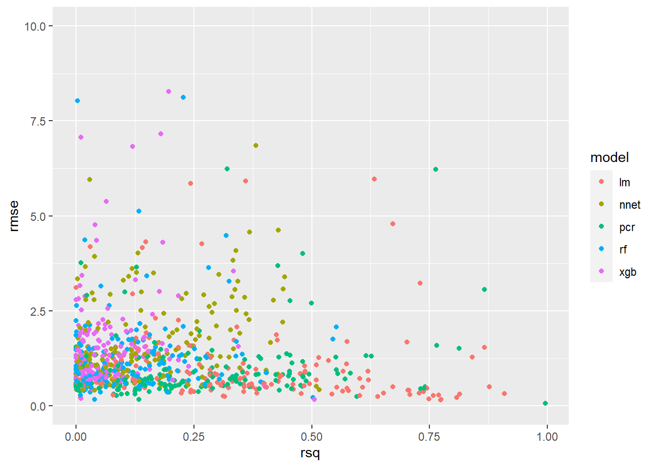
ggplotly(ggplot(plot_scores, aes(x=rsq, y=rmse, color = model, symbol = symbol)) +
           geom_point() +
           ylim(c(0,10)),
         tooltip = c("model", "symbol", "rmse", "rsq"))
The additional tooltip argument was passed to ggpltoly() to specify the label when hovering over the individual points.
8.7.3 Results by the Cryptocurrency
We can use the facet_wrap() function from ggplot2 to create an individual chart for each cryptocurrency:
ggplot(plot_scores, aes(x=rsq, y=rmse, color = model)) +
  geom_point() +
  geom_smooth() +
  ylim(c(0,10)) +
  facet_wrap(~symbol)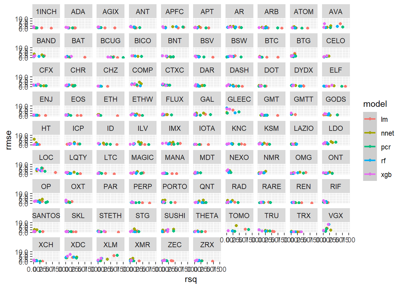
Every 12 hours once this document reaches this point, the results are saved to GitHub using the pins package (which we used to read in the data at the start), and a separate script running on a different server creates the complete dataset in our database over time. You won’t be able to run the code shown below (nor do you have a reason to):
8.8 Interactive Dashboard
Use the interactive app below to explore the results over time by the individual cryptocurrency. Use the filters on the left sidebar to visualize the results you are interested in:
If you have trouble viewing the embedded dashboard you can open it here instead: https://predictcrypto.shinyapps.io/tutorial_latest_model_summary/
The default view shows the holdout results for all models. Another interesting comparison to make is between the holdout and the test set for fewer models (2 is ideal).
8.9 Visualizations - Historical Metrics
We can pull the same data into this R session using the pin_get() function:
The data is limited to metrics for runs from the past 30 days and includes new data every 12 hours. Using the tools we used in the data prep section, we can answer a couple more questions.
8.9.1 Best Models
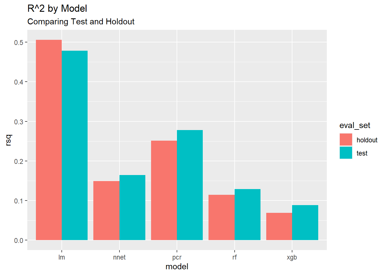
Overall, which model has the best metrics for all runs from the last 30 days?
8.9.1.1 Summarize the data
# First create grouped data
best_models <- group_by(metrics_historical, model, eval_set)
# Now summarize the data
best_models <- summarize(best_models,
                         rmse = mean(rmse, na.rm=T),
                         rsq  = mean(rsq, na.rm=T))
# Show results
best_models
## # A tibble: 10 x 4
## # Groups: model [5]
## model eval_set rmse rsq
## <chr> <chr> <dbl> <dbl>
## 1 lm holdout 15.5 0.506
## 2 lm test 4.07 0.478
## 3 nnet holdout 4.31 0.149
## 4 nnet test 4.63 0.164
## 5 pcr holdout 2.72 0.252
## 6 pcr test 2.92 0.278
## 7 rf holdout 3.96 0.114
## 8 rf test 3.83 0.129
## 9 xgb holdout 5.01 0.0693
## 10 xgb test 4.56 0.0885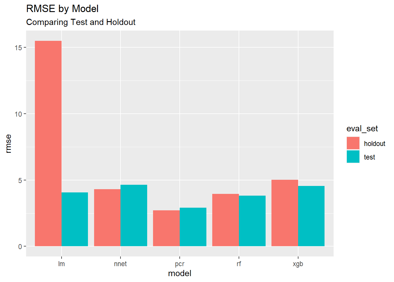
8.9.2 Most Predictable Cryptocurrency
Overall, which cryptocurrency has the best metrics for all runs from the last 30 days?
8.9.2.1 Summarize the data
# First create grouped data
predictable_cryptos <- group_by(metrics_historical, symbol, eval_set)
# Now summarize the data
predictable_cryptos <- summarize(predictable_cryptos,
                         rmse = mean(rmse, na.rm=T),
                         rsq  = mean(rsq, na.rm=T))
# Arrange from most predictable (according to R^2) to least
predictable_cryptos <- arrange(predictable_cryptos, desc(rsq))
# Show results
predictable_cryptos
## # A tibble: 178 x 4
## # Groups: symbol [89]
## symbol eval_set rmse rsq
## <chr> <chr> <dbl> <dbl>
## 1 NAV test 3.30 0.434
## 2 POA holdout 4.60 0.423
## 3 CUR holdout 6.09 0.410
## 4 CND test 1.84 0.374
## 5 CND holdout 5.24 0.360
## 6 SEELE holdout 8.88 0.355
## 7 ADXN test 9.26 0.348
## 8 RCN test 5.03 0.337
## 9 BTC test 1.32 0.331
## 10 SUN holdout 3.17 0.330
## # ... with 168 more rowsShow the top 15 most predictable cryptocurrencies (according to the \(R^2\)) using the formattable package (Ren and Russell 2016) to color code the cells:
formattable(head(predictable_cryptos ,15),
            list(rmse = color_tile("#71CA97", "red"),
rsq = color_tile("firebrick1", "#71CA97")))| symbol | eval_set | rmse | rsq |
|---|---|---|---|
| NAV | test | 3.299791 | 0.4338237 |
| POA | holdout | 4.596582 | 0.4229192 |
| CUR | holdout | 6.088416 | 0.4098434 |
| CND | test | 1.835020 | 0.3737691 |
| CND | holdout | 5.238670 | 0.3601346 |
| SEELE | holdout | 8.876745 | 0.3548372 |
| ADXN | test | 9.263022 | 0.3478368 |
| RCN | test | 5.030197 | 0.3367737 |
| BTC | test | 1.321379 | 0.3307333 |
| SUN | holdout | 3.172350 | 0.3299285 |
| AAB | test | 39.511003 | 0.3262746 |
| ETH | test | 1.721290 | 0.3197170 |
| LTC | test | 2.102832 | 0.3189001 |
| LEO | test | 1.695632 | 0.3166553 |
| RCN | holdout | 7.564985 | 0.3130917 |
8.9.3 Accuracy Over Time
8.9.3.1 Summarize the data
# First create grouped data
accuracy_over_time <- group_by(metrics_historical, date_utc)
# Now summarize the data
accuracy_over_time <- summarize(accuracy_over_time,
                                rmse = mean(rmse, na.rm=T),
                                rsq  = mean(rsq, na.rm=T))
# Ungroup data
accuracy_over_time <- ungroup(accuracy_over_time)
# Convert date/time
accuracy_over_time$date_utc <- anytime(accuracy_over_time$date_utc)
# Show results
accuracy_over_time
## # A tibble: 30 x 3
## date_utc rmse rsq
## <dttm> <dbl> <dbl>
## 1 2021-01-12 00:00:00 4.05 0.241
## 2 2021-01-13 00:00:00 4.29 0.236
## 3 2021-01-14 00:00:00 4.06 0.251
## 4 2021-01-16 00:00:00 4.25 0.214
## 5 2021-01-17 00:00:00 3.78 0.199
## 6 2021-01-18 00:00:00 3.88 0.212
## 7 2021-01-19 00:00:00 3.86 0.204
## 8 2021-01-20 00:00:00 4.65 0.207
## 9 2021-01-21 00:00:00 3.41 0.222
## 10 2021-01-22 00:00:00 4.05 0.231
## # ... with 20 more rows8.9.3.2 Plot RMSE
Remember, for RMSE the lower the score, the more accurate the models were.
ggplot(accuracy_over_time, aes(x = date_utc, y = rmse, group = 1)) +
  # Plot RMSE over time
  geom_point(color = 'red', size = 2) +
  geom_line(color = 'red', size = 1)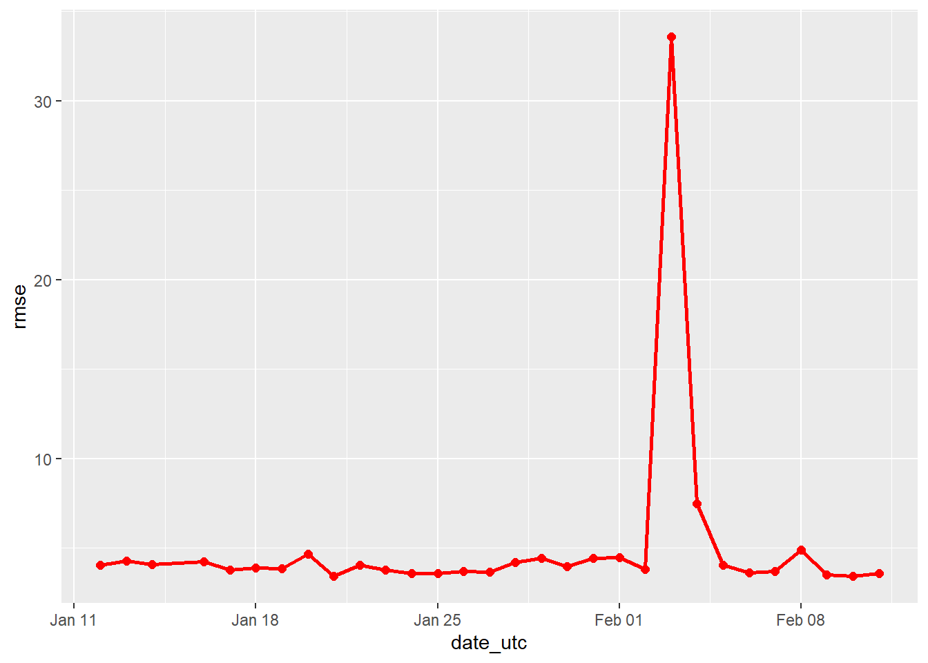
8.9.3.3 Plot R^2
For the R^2 recall that we are looking at the correlation between the predictions made and what actually happened, so the higher the score the better, with a maximum score of 1 that would mean the predictions were 100% correlated with each other and therefore identical.
ggplot(accuracy_over_time, aes(x = date_utc, y = rsq, group = 1)) +
  # Plot R^2 over time
  geom_point(aes(x = date_utc, y = rsq), color = 'dark green', size = 2) +
  geom_line(aes(x = date_utc, y = rsq), color = 'dark green', size = 1)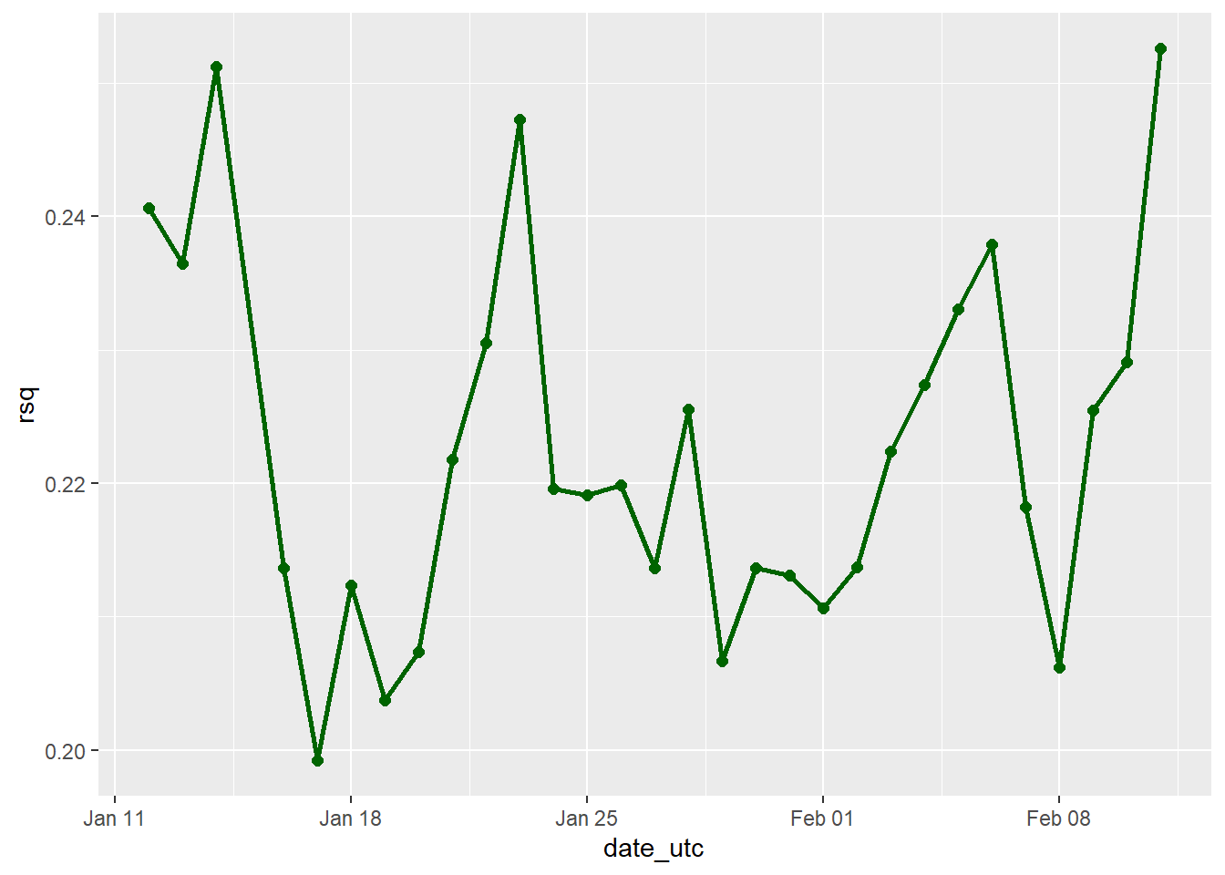
Refer back to the interactive dashboard to take a more specific subset of results instead of the aggregate analysis shown above.
References
Ren, Kun, and Kenton Russell. 2016. Formattable: Create Formattable Data Structures. https://CRAN.R-project.org/package=formattable.